import numpy as np
from affine import Affine

from planetarypy.geo import (
    pixel_to_xy,
    xy_to_pixel,
    pixel_to_lonlat,
    lonlat_to_pixel,
    xy_to_lonlat,
    lonlat_to_xy,
    image_azimuth,
    image_azimuth_cw_from_right,
    pixel_resolution,
)Geospatial Utilities for Planetary Images
The planetarypy.geo module provides coordinate transforms for planetary image data — converting between pixel coordinates, map-projected coordinates, and geographic (lon/lat) coordinates.
It is built on rasterio and pyproj (no GDAL required) and works with both Earth and planetary CRS (Mars, Moon, etc.).
Pixel ↔︎ Map Coordinates
Every georeferenced image has an affine transform that maps pixel (sample, line) to map-projected (x, y) coordinates. This is a simple 2×3 matrix — no CRS needed.
# A Mars equirectangular image: 200 m/pixel, origin at x=-50km, y=100km
transform = Affine(200.0, 0.0, -50000.0,
                   0.0, -200.0, 100000.0)

# Pixel (100, 50) → map coordinates
x, y = pixel_to_xy(transform, sample=100, line=50)
print(f"Pixel (100, 50) → x={x:.0f} m, y={y:.0f} m")
Pixel (100, 50) → x=-29900 m, y=89900 m# And back: map coordinates → pixel
s, l = xy_to_pixel(transform, x, y)
print(f"x={x:.0f}, y={y:.0f} → pixel ({s:.0f}, {l:.0f})")x=-29900, y=89900 → pixel (100, 50)# Works with arrays too — convert an entire grid of pixels
samples = np.array([0, 50, 100, 150, 200])
lines = np.array([0, 0, 0, 0, 0])
xs, ys = pixel_to_xy(transform, samples, lines)
print("Samples:", samples)
print("X coords:", xs)Samples: [ 0 50 100 150 200]
X coords: [-49900. -39900. -29900. -19900. -9900.]# Get pixel resolution from the transform
res_x, res_y = pixel_resolution(transform)
print(f"Pixel resolution: {res_x:.0f} × {res_y:.0f} m")Pixel resolution: 200 × 200 mMap Coordinates ↔︎ Geographic (Lon/Lat)
To go from map-projected coordinates to lon/lat (or vice versa), you need a CRS. The geo module uses pyproj under the hood and automatically derives the correct geographic CRS from the projected CRS — so it works for any planetary body, not just Earth.
Planetary bodies use IAU CRS codes (supported by GDAL, ISIS, and pyproj). The convention is IAU_2015:{body_id}XX where the body ID follows the NAIF convention (e.g. Mars = 499, Moon = 301).
from pyproj import CRS as ProjCRS

# The old way: raw proj4 string (works but fragile, easy to get radius wrong)
mars_manual = ProjCRS.from_proj4("+proj=eqc +lat_ts=0 +lon_0=0 +R=3396190 +units=m")
print(f"Manual proj4: '{mars_manual.name}'")  # → 'unknown' — no metadata!

# The better way: IAU 2015 CRS codes
# 49910 = Mars (NAIF body 499) + equirectangular sphere ocentric (suffix 10)
mars_equirect = ProjCRS.from_authority("IAU_2015", 49910)
print(f"IAU code:     '{mars_equirect.name}'")

# The proj4 CRS is just math with no identity — pyproj can't even name it.
# The IAU code carries body name, projection, and datum. It's what GDAL,
# ISIS, and the PDS4 standard use. Always prefer IAU codes.

# Both produce the same coordinates:
lon, lat = xy_to_lonlat(mars_equirect, x=1_000_000, y=500_000)
print(f"\nx=1000km, y=500km → lon={lon:.2f}°, lat={lat:.2f}°")
Manual proj4: 'unknown'
IAU code: 'Mars (2015) - Sphere / Ocentric / Equirectangular, clon = 0'
x=1000km, y=500km → lon=16.87°, lat=8.44°# Roundtrip: lon/lat → projected → lon/lat
x2, y2 = lonlat_to_xy(mars_equirect, lon=45.0, lat=-10.0)
lon2, lat2 = xy_to_lonlat(mars_equirect, x2, y2)
print(f"lon=45°, lat=-10° → x={x2:.0f}, y={y2:.0f} → lon={lon2:.4f}°, lat={lat2:.4f}°")lon=45°, lat=-10° → x=2667361, y=-592747 → lon=45.0000°, lat=-10.0000°# Mars north polar stereographic — IAU code 49930
mars_npole = ProjCRS.from_authority("IAU_2015", 49930)
print(f"CRS: {mars_npole.name}")
x, y = lonlat_to_xy(mars_npole, lon=45.0, lat=85.0)
print(f"North polar region: lon=45°, lat=85° → x={x:.0f} m, y={y:.0f} m")
lon_back, lat_back = xy_to_lonlat(mars_npole, x, y)
print(f"Back to geographic: lon={lon_back:.4f}°, lat={lat_back:.4f}°")
# Some useful IAU 2015 codes:
print("\nCommon planetary CRS codes:")
for code, desc in [(49900, "Mars geographic"),
(49910, "Mars equirectangular"),
(49930, "Mars north polar"),
(30100, "Moon geographic"),
(30110, "Moon equirectangular"),
(60600, "Enceladus geographic")]:
c = ProjCRS.from_authority("IAU_2015", code)
print(f" IAU_2015:{code} → {c.name}")CRS: Mars (2015) - Sphere / Ocentric / North Polar
North polar region: lon=45°, lat=85° → x=209701 m, y=-209701 m
Back to geographic: lon=45.0000°, lat=85.0000°
Common planetary CRS codes:
IAU_2015:49900 → Mars (2015) - Sphere / Ocentric
IAU_2015:49910 → Mars (2015) - Sphere / Ocentric / Equirectangular, clon = 0
IAU_2015:49930 → Mars (2015) - Sphere / Ocentric / North Polar
IAU_2015:30100 → Moon (2015) - Sphere / Ocentric
IAU_2015:30110 → Moon (2015) - Sphere / Ocentric / Equirectangular, clon = 0
IAU_2015:60600 → Titan (2015) - Sphere / OcentricPixel ↔︎ Lon/Lat (Full Chain)
The pixel_to_lonlat and lonlat_to_pixel functions combine the affine transform and CRS reprojection into a single call. They accept a rioxarray DataArray directly — because rioxarray stores both the affine transform and the CRS as metadata inside the DataArray (in the spatial_ref coordinate). This means the DataArray is fully self-describing: you don’t need to pass the CRS or transform separately.
Let’s create a synthetic Mars image to demonstrate:
import math

import xarray as xr
import rioxarray  # noqa: F401 — activates .rio accessor

# Create a synthetic 500x500 "image" over Gale Crater region on Mars
# Equirectangular projection, 200 m/pixel
# Centered roughly on Gale Crater: lon=137.4°, lat=-4.6°
pixel_size = 200  # meters
nx, ny = 500, 500

# Affine transform: origin at the upper-left corner in projected coords
# For Mars equirectangular: x = lon * R * pi/180, y = lat * R * pi/180
R_mars = 3396190  # meters
center_x = 137.4 * math.pi / 180 * R_mars
center_y = -4.6 * math.pi / 180 * R_mars
origin_x = center_x - (nx / 2) * pixel_size
origin_y = center_y + (ny / 2) * pixel_size

transform = Affine(pixel_size, 0.0, origin_x,
                   0.0, -pixel_size, origin_y)

# Build coordinate arrays from the transform (pixel centers)
xs = origin_x + (np.arange(nx) + 0.5) * pixel_size
ys = origin_y - (np.arange(ny) + 0.5) * pixel_size

# Create DataArray with proper coordinates and CRS
data = np.random.rand(ny, nx).astype(np.float32)
da = xr.DataArray(data, dims=["y", "x"], coords={"x": xs, "y": ys})
da = da.rio.set_spatial_dims(x_dim="x", y_dim="y")
da = da.rio.write_crs("IAU_2015:49910")
da = da.rio.write_transform(transform)

print(f"Image: {nx}×{ny} pixels, {pixel_size} m/pixel")
print(f"CRS: {da.rio.crs}")
print(f"Bounds: {da.rio.bounds()}")
Image: 500×500 pixels, 200 m/pixel
CRS: PROJCS["Mars (2015) - Sphere / Ocentric / Equirectangular, clon = 0",GEOGCS["Mars (2015) - Sphere / Ocentric",DATUM["Mars (2015) - Sphere",SPHEROID["Mars (2015) - Sphere",3396190,0,AUTHORITY["IAU","49900"]],AUTHORITY["IAU","49900"]],PRIMEM["Reference Meridian",0,AUTHORITY["IAU","49900"]],UNIT["degree",0.0174532925199433,AUTHORITY["EPSG","9122"]],AUTHORITY["IAU","49900"]],PROJECTION["Equirectangular"],PARAMETER["standard_parallel_1",0],PARAMETER["central_meridian",0],PARAMETER["false_easting",0],PARAMETER["false_northing",0],UNIT["metre",1,AUTHORITY["EPSG","9001"]],AXIS["Easting",EAST],AXIS["Northing",NORTH],AUTHORITY["IAU","49910"]]
Bounds: (8094343.439702274, -322663.6086072086, 8194343.439702274, -222663.6086072086)# The DataArray carries all the geo metadata — inspect it:
print(f"Transform: {da.rio.transform()}")
print(f"CRS: {da.rio.crs}")
print("Stored in: da.coords['spatial_ref']")
print("\nThis is why pixel_to_lonlat(da, ...) works without extra arguments —")
print("the DataArray knows its own coordinate system.")Is a raster’s CRS projected?
is_projected reports whether a raster’s CRS is projected (map units like metres) or geographic (degrees) — handy before assuming planar geometry. It accepts a file path, a rasterio dataset, or a rioxarray DataArray, and works on any GDAL-readable format.
from planetarypy.geo import is_projected

# `da` is map-projected (Mars equirectangular) → its CRS is projected
print(f"da CRS projected? {is_projected(da)}")
# pixel_to_lonlat: where is the center pixel on Mars?
center_sample, center_line = nx // 2, ny // 2
lon, lat = pixel_to_lonlat(da, sample=center_sample, line=center_line)
print(f"Center pixel ({center_sample}, {center_line}) → lon={lon:.2f}°, lat={lat:.2f}°")
print("(Expected: ~137.4°, ~-4.6° — Gale Crater)")
# Works with arrays — get lon/lat for the four corners
corners_s = np.array([0, nx-1, 0, nx-1])
corners_l = np.array([0, 0, ny-1, ny-1])
lons, lats = pixel_to_lonlat(da, sample=corners_s, line=corners_l)
for label, lo, la in zip(["UL", "UR", "LL", "LR"], lons, lats):
print(f" {label}: lon={lo:.2f}°, lat={la:.2f}°")from planetarypy.geo import is_within
# lonlat_to_pixel: which pixel is Gale Crater's central peak?
# (Aeolis Mons / Mt Sharp: lon=137.85°, lat=-5.08°)
s, l = lonlat_to_pixel(da, lon=137.85, lat=-5.08)
print(f"Mt Sharp (137.85°, -5.08°) → pixel ({s:.0f}, {l:.0f})")
# Bounds check
print(f" Within image: {is_within(da, lon=137.85, lat=-5.08)}")
# Something far away
print(f" Olympus Mons within image: {is_within(da, lon=226.2, lat=18.65)}")
# Roundtrip check
lon_rt, lat_rt = pixel_to_lonlat(da, sample=s, line=l)
print(f" Roundtrip: lon={lon_rt:.4f}°, lat={lat_rt:.4f}°")Mt Sharp (137.85°, -5.08°) → pixel (383, 392)
Within image: True
Olympus Mons within image: False
Roundtrip: lon=137.8504°, lat=-5.0808°With a real planetary image file, it’s even simpler — rioxarray reads the transform and CRS from the file:
import rioxarray as rxr

da = rxr.open_rasterio("my_hirise_dtm.tif").isel(band=0)

# Where is pixel (1000, 2000)?
lon, lat = pixel_to_lonlat(da, sample=1000, line=2000)

# Which pixel is Olympus Mons summit?
s, l = lonlat_to_pixel(da, lon=226.2, lat=18.65)
Image Azimuth Angles
Two conventions are provided for measuring angles between points in image space:
| Function | Zero direction | Rotation | Use case |
|---|---|---|---|
image_azimuth |
North (up) | Clockwise | Standard planetary science |
image_azimuth_cw_from_right |
East (right, 3 o’clock) | Clockwise | HiRISE rotation angles |
# Standard planetary science: clockwise from north
# A point directly to the east → 90°
az = image_azimuth(100, 100, 150, 100)
print(f"East: {az:.0f}°")

# Point to the southwest → 225°
az = image_azimuth(100, 100, 80, 120)
print(f"Southwest: {az:.0f}°")
East: 90°
Southwest: 225°# HiRISE convention: clockwise from 3 o'clock
# A point directly downward → 90°
az = image_azimuth_cw_from_right(100, 100, 100, 150)
print(f"Down (HiRISE): {az:.0f}°")
# A point directly upward → 270°
az = image_azimuth_cw_from_right(100, 100, 100, 50)
print(f"Up (HiRISE): {az:.0f}°")Down (HiRISE): 90°
Up (HiRISE): 270°The Point Class
Why a custom Point?
Existing geospatial libraries each cover part of the planetary image workflow but none cover it all:
| Library | What it does | What it doesn’t do |
|---|---|---|
Shapely Point |
Geometry operations (intersect, buffer, distance) | No CRS, no pixel transforms, no image bounds |
pyproj Transformer |
CRS reprojection | No point object — bare tuples only |
| rasterio | rowcol() / xy() pixel↔︎map |
No point class, no lon/lat, no bounds check |
| geopandas | CRS-aware geometries | Heavyweight for a single point |
The planetarypy Point combines what planetary scientists actually need in one object: create a point from lon/lat (or pixel coordinates), project it, check if it’s in an image, compute azimuths — all CRS-aware, all working with IAU planetary bodies.
For GIS interop, you can always hand off to Shapely:
from shapely.geometry import Point as ShapelyPoint
shapely_pt = ShapelyPoint(p.lon, p.lat)
from planetarypy.geo import Point
# Create a point from geographic coordinates
mt_sharp = Point(lon=137.85, lat=-5.08, crs="IAU_2015:49900")
mt_sharpPoint(lon=137.8500, lat=-5.0800, crs='Mars (2015) - Sphere / Ocentric')# Project to Mars equirectangular
x, y = mt_sharp.to_xy("IAU_2015:49910")
print(f"Mt Sharp projected: x={x:.0f} m, y={y:.0f} m")
# Check if it's within our synthetic Gale Crater image
print(f"Within image: {mt_sharp.is_within(da)}")
# Get pixel coordinates in the image
s, l = mt_sharp.to_pixel(da)
print(f"Pixel: ({s:.0f}, {l:.0f})")Mt Sharp projected: x=8171017 m, y=-301115 m
Within image: True
Pixel: (383, 392)# Create a point from pixel coordinates — lon/lat auto-resolved
center = Point(sample=250, line=250, source=da)
print(f"Image center: {center}")
# Azimuth from center to Mt Sharp
mt_sharp_px = Point(lon=137.85, lat=-5.08, source=da)
az = center.azimuth_to(mt_sharp_px)
print(f"Azimuth from center to Mt Sharp: {az:.1f}° (CW from north)")Image center: Point(lon=137.4017, lat=-4.6017, sample=250, line=250, crs='Mars (2015) - Sphere / Ocentric / Equirectangular, clon = 0')
Azimuth from center to Mt Sharp: 136.9° (CW from north)# Point works for any location — check Olympus Mons is NOT in our image
olympus = Point(lon=226.2, lat=18.65, crs="IAU_2015:49900")
print(f"Olympus Mons within Gale image: {olympus.is_within(da)}")Olympus Mons within Gale image: False# Hand off to Shapely for GIS operations
shapely_pt = mt_sharp.to_shapely()
print(f"Shapely: {shapely_pt}")
print(f"Type: {type(shapely_pt).__module__}.{type(shapely_pt).__name__}")
shapely_pt # renders as SVG in JupyterShapely: POINT (137.85 -5.08)
Type: shapely.geometry.point.Point
Sun Direction Indicator
The planetarypy.plotting module provides add_sun_indicator and imshow_with_sun for displaying images with a sun direction overlay. The indicator expects the solar azimuth clockwise from image top (CW-from-top).
Azimuth conventions
Different data sources use different zero directions:
| Source | Convention | Zero direction | Convert to CW-from-top |
|---|---|---|---|
planetarypy.plotting |
CW from top | Up (12 o’clock) | Use directly |
HiRISE index (SUB_SOLAR_AZIMUTH) |
CW from right | Right (3 o’clock) | (az + 90) % 360 |
| Standard geographic | CW from north | North | Depends on image orientation |
The HiRISE convention (CW from 3 o’clock) is documented in the HiRISE EDR/RDR SIS and the ASU HiRISE glossary. Both SUB_SOLAR_AZIMUTH and NORTH_AZIMUTH use this convention.
import matplotlib.pyplot as plt
from planetarypy.plotting import imshow_with_sun, imshow_gray, add_sun_indicator
Verification with real HiRISE data
Let’s verify the sun indicator against a real HiRISE RDR browse image with clearly visible shadows. We’ll use ESP_013807_2035 — a mid-latitude observation with prominent crater shadows.
The browse image (.abrowse.jpg) is the map-projected RDR, so it uses the RDR index metadata. In HiRISE’s equirectangular RDRs, NORTH_AZIMUTH=270° (CW from right), meaning north has been rotated to the top of the image.
from planetarypy.instruments.mro.hirise import get_browse, get_metadata, sun_azimuth_from_top

# Look up solar geometry from the HiRISE RDR index
meta = get_metadata("ESP_013807_2035_RED")

print(f"Observation: {meta['PRODUCT_ID']}")
print(f"SUB_SOLAR_AZIMUTH: {meta['SUB_SOLAR_AZIMUTH']:.1f}° (CW from 3 o'clock)")
print(f"NORTH_AZIMUTH:     {meta['NORTH_AZIMUTH']:.1f}° (CW from 3 o'clock)")
print(f"INCIDENCE_ANGLE:   {meta['INCIDENCE_ANGLE']:.1f}°")
print(f"MAP_PROJECTION:    {meta['MAP_PROJECTION_TYPE']}")
Observation: ESP_013807_2035_RED
SUB_SOLAR_AZIMUTH: 129.3° (CW from 3 o'clock)
NORTH_AZIMUTH: 270.0° (CW from 3 o'clock)
INCIDENCE_ANGLE: 56.0°
MAP_PROJECTION: EQUIRECTANGULARimport matplotlib.image as mpimg
# Download the clean (unannotated) browse — better for image analysis
# Equivalent to: plp hibrowse --clean ESP_013807_2035_RED
browse_path = get_browse("ESP_013807_2035_RED", annotated=False)
img = mpimg.imread(str(browse_path))
print(f"Browse image: {browse_path.name}")
print(f"Size: {img.shape[1]}×{img.shape[0]} pixels")Browse image: ESP_013807_2035_RED.browse.jpg
Size: 2048×5959 pixels# imshow_gray: quick display with automatic percentile stretch
# HiRISE images are well-behaved — a gentle 0.5-99.5 stretch is usually enough
ax = imshow_gray(img, stretch="0.5,99.5", title="ESP_013807_2035 — full browse")
plt.show()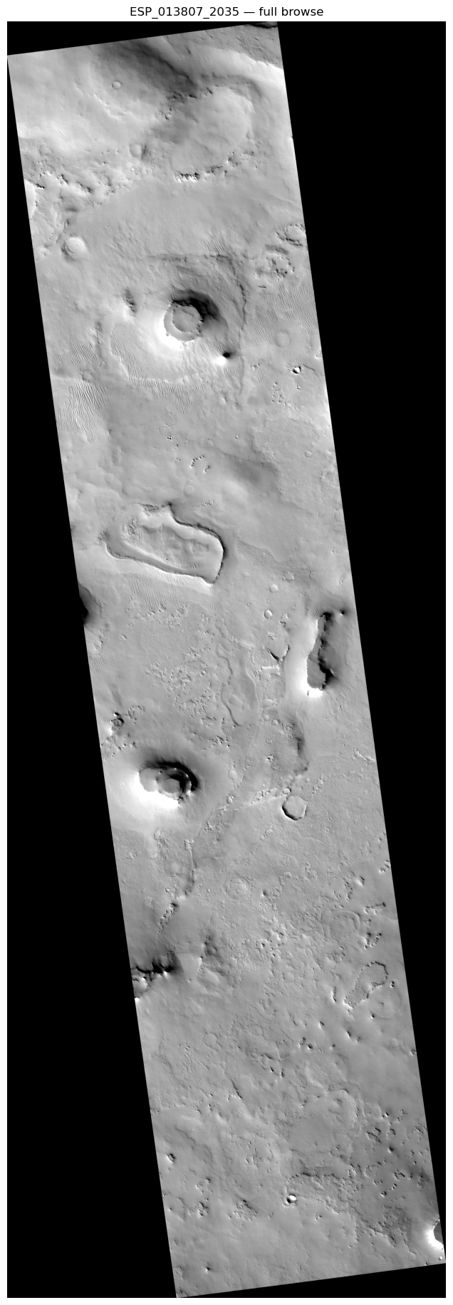
# Convert HiRISE azimuth to our plotting convention in one call
sun_az_from_top = sun_azimuth_from_top("ESP_013807_2035_RED")

print(f"HiRISE SUB_SOLAR_AZIMUTH: {meta['SUB_SOLAR_AZIMUTH']:.1f}° (CW from right)")
print(f"Converted to CW from top: {sun_az_from_top:.1f}°")
print("\nShadows should point AWAY from the sun indicator.")
HiRISE SUB_SOLAR_AZIMUTH: 129.3° (CW from right)
Converted to CW from top: 219.3°
Shadows should point AWAY from the sun indicator.# Crop a window with clear crater shadows (middle of the image)
window = img[1500:2500, 400:1600]
fig, ax = plt.subplots(figsize=(10, 8))
imshow_with_sun(window, sun_az_from_top, stretch="0.5,99.5",
title=f"ESP_013807_2035 — SUB_SOLAR_AZIMUTH={meta['SUB_SOLAR_AZIMUTH']:.1f}° → {sun_az_from_top:.1f}° from top",
ax=ax)
fig.tight_layout()
plt.show()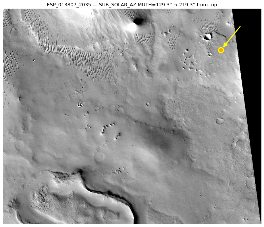
# add_sun_indicator can be added to any existing axes
# Useful when you've already built a plot with other overlays
fig, ax = plt.subplots(figsize=(10, 8))
ax.imshow(window, cmap="gray")
ax.set_title("Manual plot + sun indicator added separately")
add_sun_indicator(ax, sun_az_from_top, position="upper left")
plt.show()
Text(0.5, 1.0, 'Manual plot + sun indicator added separately')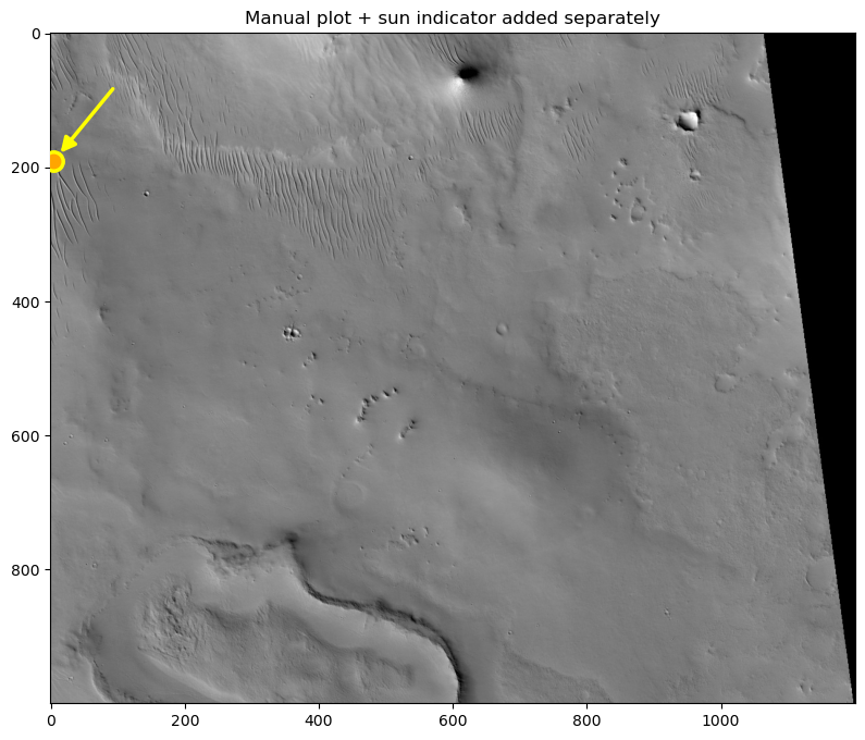
Next Steps
We are planning to incorporate a planetarypy CRS module written by Christian Tai Udovicic that will enable easy access to all major solar system CRSs.
Other planned features:
- Verify the sun indicator convention for unprojected EDR images (RDR convention is verified:
(hirise_az + 90) % 360) - Independent sun azimuth calculation via SPICE to validate index values
- Automatic sun indicator from PDS index metadata (no manual conversion)
- Sun indicator support for CTX images (using
SUB_SOLAR_AZIMUTHfrom CTX index)