
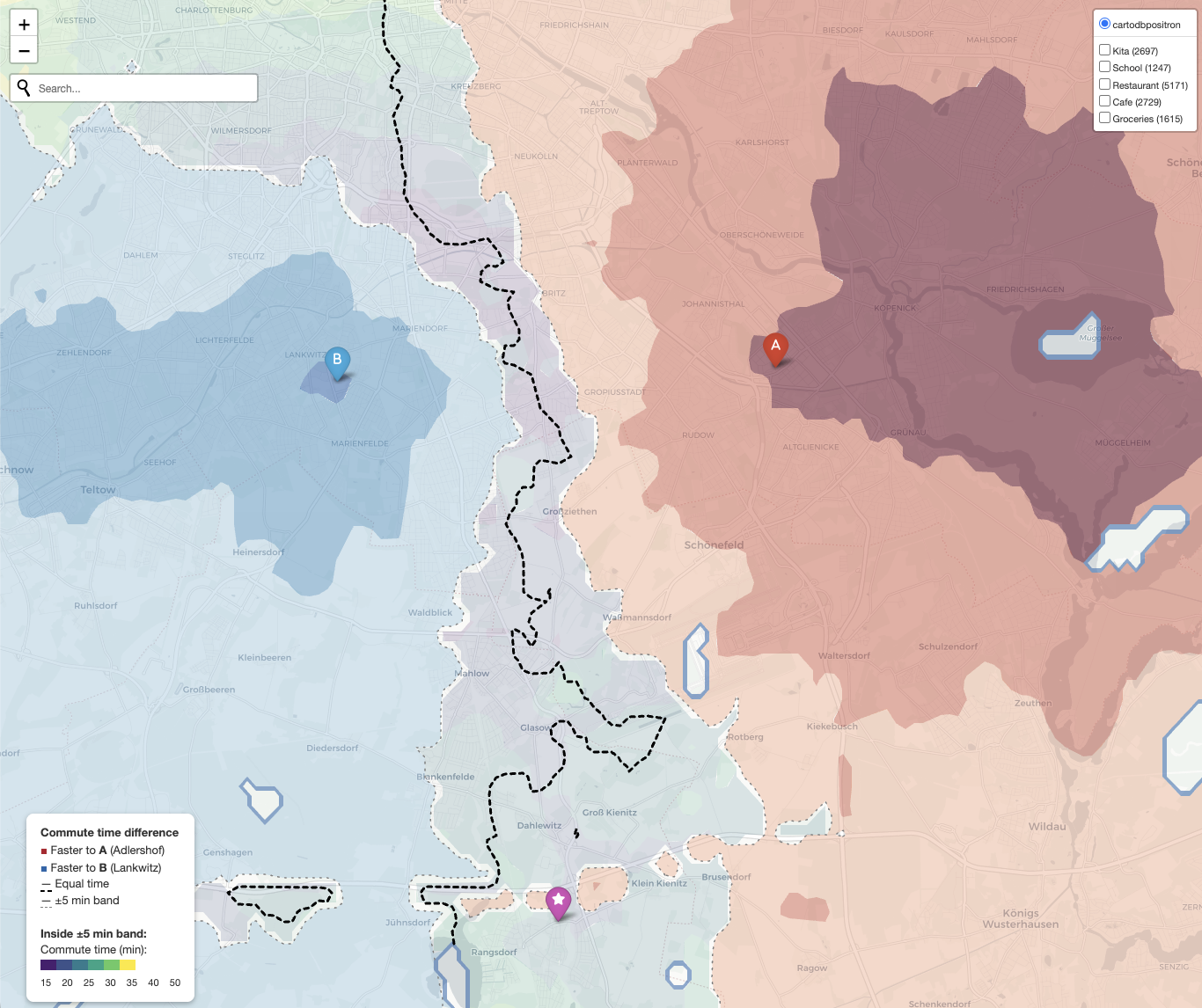
When two people in a household work in different parts of a city, picking where to live is an optimization problem the usual house-hunting tools don’t solve. Single-origin isochrones are everywhere — “20 minutes from this address” — but the thing I actually wanted to see was the set of neighborhoods where both commutes come out roughly equal. So I wrote it.
The approach is straightforward:
- Lay down a regular grid over the city’s bounding box
- Ask OpenRouteService (ORS) for driving time from every grid point to each workplace
- Compute the scalar field
t_A − t_B, extract the zero contour, and draw a ±5 min tolerance band on either side - Fill the rest of the map with a red↔︎blue gradient so you can also see who is faster by how much in the regions that aren’t fair game
Inside the decision zone, a second viridis colormap shows the actual commute time, so you can distinguish a 20-min equal-commute spot from a 40-min one. On top, toggleable OSM overlays show kitas, schools, restaurants, cafes, and supermarkets. Clicking a POI marker pops up driving, cycling, and walking times to pinned addresses of interest.
Gotchas worth writing down
ORS snapping will lie to you. When you send a grid point that lands in a lake, a forest, or a military airfield, ORS doesn’t return NaN — it silently snaps the point to the nearest routable road, possibly kilometers away, and returns the travel time from there. The result is phantom contours wrapping around Rangsdorfer See. The fix is to set resolve_locations: true in the matrix request, read the returned snapped_distance per source, and drop any grid point that got snapped more than ~400 m. In Berlin this removes ~13% of the grid.
Water is still worth masking explicitly. Even after the snap filter, a pass through the OSM natural=water polygons via Overpass catches everything that slipped through (floating pontoons, narrow canals, edge cases) and makes the logic obvious.
Linear interpolation > cubic. scipy.interpolate.griddata with method="cubic" overshoots near sparse data and conjures up small closed contours that look like artifacts because they are. Switching to linear and tagging fine-grid cells too far from any valid source as no-data gives a cleaner picture of where you have reliable data and where you don’t. Forests and airfields become visible gaps — which is exactly what they should be.
Cache everything. First run is ~30s of ORS matrix calls, plus Overpass POIs and water polygons. Every subsequent run is seconds because all the expensive bits land in .npz / .json files fingerprinted by the config. Refusing to cache empty results (which happens when Overpass mirrors fall over) saves a lot of “why is my map blank” debugging.
Links
The code is on GitHub and citable via Zenodo:
- Repo: github.com/michaelaye/equal-commute
- DOI: 10.5281/zenodo.19520780
- License: MIT
It’s Berlin-specific in the default config, but the only things pinning it to one city are the bounding box and the two workplace coordinates. If you have the same problem in Munich or Paris, edit six lines.